
Dr. Maryam Mirhadi, PMP, PSP | Principal Consultant
One of the tools that can be used to assess the time-phased projected number of activities scheduled over the course of a project is the schedule activity density analysis. A schedule activity density histogram represents the cumulative number of activities that are, partly or wholly, scheduled to be performed within each time unit over the course of the project. The schedule activity density can alternatively be measured by activity-workdays scheduled per time analysis period (if activity durations are defined in days).
For instance, if a 10 and a 20 working-day activities are supposed to start and complete in a particular month, the activity-workdays for that particular month will be 30 (i.e., 10+20). If a 10 working-day activity, a 20 working-day activity, and half of an 8 working-day activity are supposed to start and complete in a particular month, the activity-workdays for that particular month will be 34 (i.e., 10+20+8/2).
As such, if a schedule activity density is high within a particular time analysis period, it can be concluded that a high number of activities are in-progress within that particular time analysis period. Therefore, it is expected that delays influence schedule activity density histograms as well because delays change the number of activities that are scheduled to be undertaken within certain time frames. Delayed work typically results in the overlapping of planned future work; therefore, delays are expected to increase the schedule’s activity density during the time frames in which planned future work will be scheduled.
Figure 1 provides an example schedule activity density histogram in which the schedule activity density is shown by the number of activity-workdays scheduled per time analysis period (i.e., monthly periods).
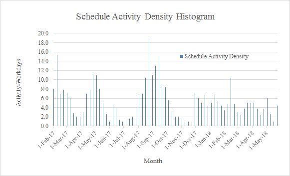
Figure 1. An example schedule activity density histogram
A review of Figure 1 indicates that the schedule activity density is the highest about September 2017 in which the number of activity-workdays is at the highest point whereas, in a time analysis period such as December 2017, the number of activity-workdays is at the lowest point. This indication suggests that in or about September 2017, the highest number of in-progress activities are scheduled whereas in or about December 2017, the lowest number of in-progress activities are scheduled.
Figure 2 provides an example cumulative schedule activity density histogram in which the cumulative schedule activity density is shown by calculating the cumulative number of activity-workdays scheduled per time analysis period (i.e., monthly periods).
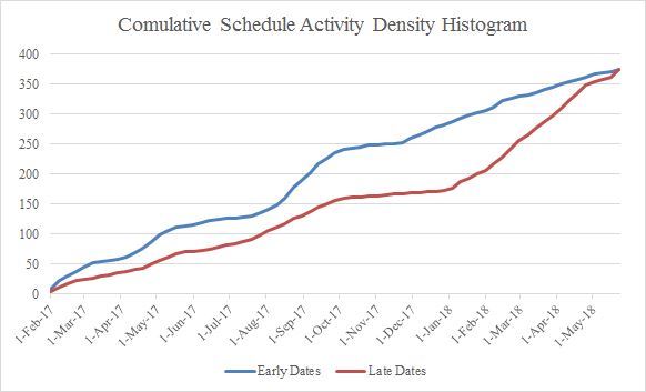
Figure 2. An example cumulative schedule activity density histogram
Two cumulative schedule activity histograms are provided in this figure. The blue histogram represents the schedule activity density for the case where the constraint type of all project activities is set to “As Soon As Possible” whereas the red histogram illustrates the schedule activity density for the case where the constraint type of all project activities is set to “As Late As Possible”. A comparison between these two histograms indicates that the cumulative number of activity-workdays scheduled per time analysis period (i.e., monthly periods) for the late chart is always less than or equal to this cumulative number for the early chart over the course of the project because setting the constraint type of all project activities to “As Late As Possible” prevents the non-critical activities from starting on their early start date and being completed on their early finish dates. This change reduces the cumulative number of activity-workdays scheduled per time analysis period (i.e., monthly periods) for the late chart and the activity density chart shifts to the right of the X-axis suggesting that more activities are being scheduled to be performed later than their original early start and finish dates.
Delayed work typically results in the overlapping of planned future work; therefore, delays are expected to increase the schedule’s activity density during the time frames in which planned future work will be scheduled. Analyzing a schedule activity density histogram is helpful in identifying the likely causes that adversely impact project schedules. For example, delaying events that prevent a set of activities from starting or finishing on-time reduce the schedule’s activity density during the time frames in which planned work cannot be performed in a timely manner but increase the schedule’s activity density during the time frames in which planned future work is supposed to be implemented. Schedule activity density histogram provides an effective way to visualize the density of schedules and obtain a better understanding of the effect of delays on the scheduled workload.
—
Our posts to the Insights page share fresh insights and seasoned advice about many project and construction management topics. To have the Insights monthly newsletter delivered automatically to your email inbox, please subscribe here.